

Introduction
As another internship season comes to a close, it’s time for our annual look under the hood at what our Software Engineering interns were up to last summer. Every year, our interns take on serious, independent projects, building systems and solutions that tackle some of our hardest trading and infrastructure problems. For this spotlight series, we’re diving into three standout projects from our 2025 Software Engineering class, all of whom recently joined HRT full-time.
And if you want to join us for the next cohort, you can apply for our upcoming summer internships here.
- SmallGrid DenseColumnar Compression by Victoria Ma
- Improving Iceberg Query Times with Z-ordering by Josh Liu
- Stall Monitor by Hadrian Reppas
SmallGrid DenseColumnar Compression
by Victoria Ma
Background
SmallGrid is a tabular pub-sub system at HRT, which started out as a summer internship project in 2021 [read more here]! It’s widely used to communicate between processes, populate GUIs, and introspect components of our trading infrastructure. Most tables today are stored as our DenseColumnarTable type, which stores columns in Arrow buffers for improved performance when most entries are non-null.
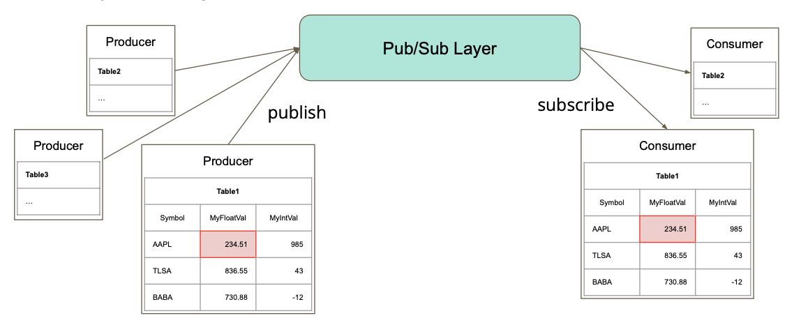
Figure 1: SmallGrid at a high level
Because of the large volume of data transmitted via SmallGrid each day, it’s important to support compression in order to reduce bandwidth usage. However, this comes at the cost of additional CPU overhead, which oftentimes isn’t tolerable for teams with strict latency requirements. The focus of my project is to support compression for DenseColumnarTable while optimizing this trade-off between bandwidth and CPU time.
General Compression Algorithms
We added compressed versions of our existing DenseColumnarTable message formats, which already cover full-state and delta updates. On the publisher’s side, we pack buffers incrementally and flush when necessary to emit compressed messages. On the subscriber’s side, partial buffers are accumulated until a full batch is available to decompress altogether.
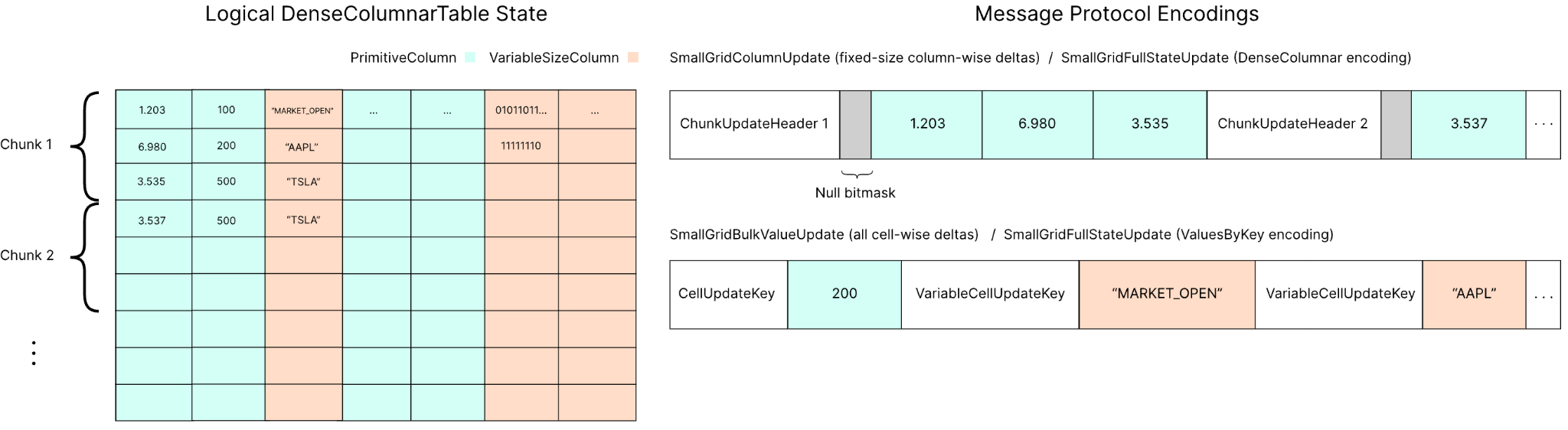
Figure 2: Example layout of a DenseColumnarTable alongside available message formats for serialized full-state and delta updates. Originally, the DenseColumnarTable publisher sends all variable-size updates cell-wise for simplicity.
After benchmarking on our common streaming data distributions, we chose to support an array of compression algorithms: LZ4, “LZ4Small” (different acceleration level), and Deflate. These provide a range of compression ratios (30-70%) with corresponding CPU time overheads (5-250% increases). We chose LZ4 in addition to the standard ZLib API specifically because LZ4 skips the traditional entropy encoding stage (such as Huffman coding). In entropy-heavy algorithms, variable-bit outputs and complex frequency tables make performance fluctuate wildly depending on how structured or random the input data is. By omitting this stage, LZ4 maintains consistent throughput and predictable execution times regardless of data distribution, which is particularly useful in lightweight, real-time compression settings.
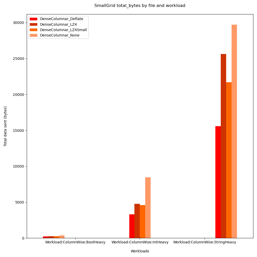
Figure 3: Total bytes across different column-wise workloads and compression algorithms.
VARIABLE-SIZE COLUMN PACKING
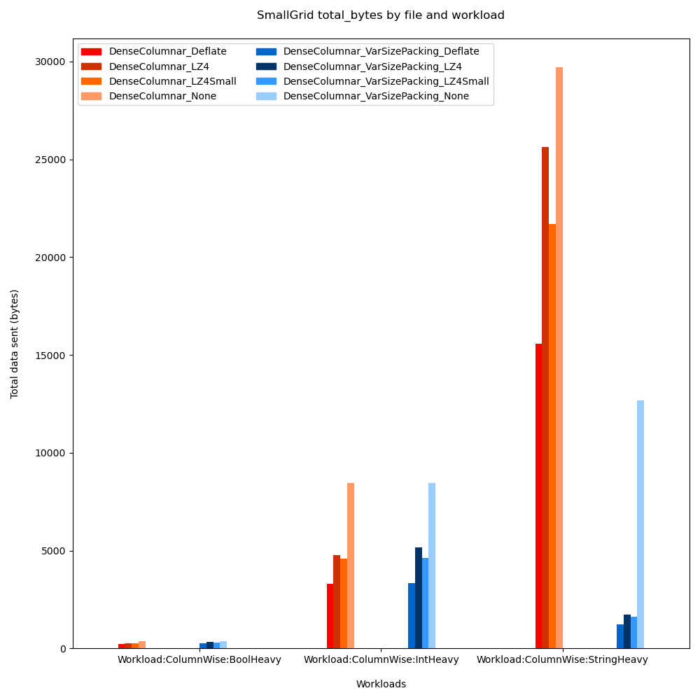
At this point though, we observed variable-sized columns (serialized cell-wise) produced larger baselines for both uncompressed and compressed sizes compared to fixed-size columns (serialized column-wise), consuming 68% more CPU time on average. We hypothesized that this was due to compression algorithms working intensely on cell-update keys rather than table values themselves. Encoding (row, column, size) tuples creates redundant key patterns that unnecessarily increase LZ4 and DEFLATE processing overhead through extra LZ77 matches, back-references, and token parsing.
And so to better support variable-size columns, we extended column-wise packing with a new pseudo-message format that uses minimal length tags to mark boundaries between variable-length elements. We purposefully reused ChunkUpdateHeader across both fixed and variable column types so they can share underlying memory buffers. Additionally, instead of forcing consumers to check for and parse length-zero tags for missing data, we encode null locations using explicit null bitmasks. This keeps zero-width values out of the payload stream and simplifies consumer-side decoding.

Figure 4: The message format for packed fixed-size columns (left) alongside packed variable-size columns (right).
Ultimately, uncompressed variable-size column packing resulted in smaller overall payloads than even compressed cell-wise updates, as grouping values by column eliminated per-cell metadata overhead. Column packing also yielded significantly higher compression ratios. Interestingly, LZ4 performed nearly as well as DEFLATE; because columnar alignment clusters homogeneous data together, repeated values (such as ticker symbols) and uniform string lengths generated long, repeating sequences of VarUpdateHeaderTags that LZ4’s simple dictionary matches easily captured. Finally, CPU overhead decreased by 57% because column-wise parsing is computationally simpler than general-purpose decompression, and total message count fell by 34% because buffer sharing aggregated multiple column updates into fewer total payloads.
Improving Iceberg Query Times with Z-ordering
By Josh Liu
At HRT, we use Apache Iceberg as our table format of choice to organize large, petabyte-scale datasets. These tables are used in many domains, from monitoring the health of our research infrastructure to post-trade analysis.
We like Iceberg because it has little vendor lock in, allowing us to substitute different query engines and customize the ingestion path. Our entire write path, in particular, is built internally to better leverage our HRT-specific distributed compute infrastructure. This means we have in-house tools to optimize datasets. Optimizations may include resorting, resharding, or adjusting row group sizes of Parquet files.
Parquet Primer
At HRT, we use Parquet as our data storage format of choice for tabular datasets. We like Parquet files for the same reasons as Iceberg: it has little vendor lock-in, high performance, and designed for storing large, complex datasets. Furthermore, Parquet is the de-facto standard for Iceberg tables.
For the scope of this post, a simple way to view a Parquet file is a list of row groups, with each group containing a batch of data:
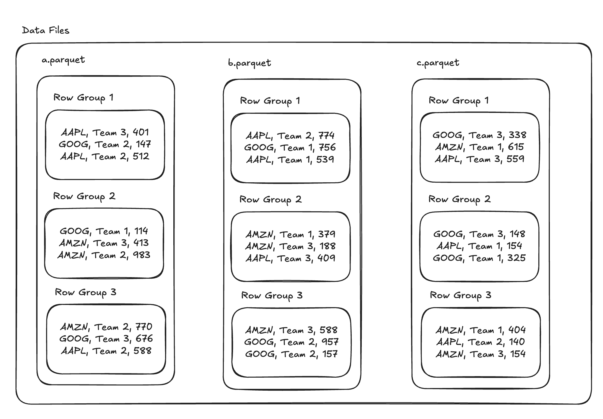
The footer of a Parquet file contains a variety of statistics about each of these row groups; most notably, it stores the minimum and maximum of each column. These statistics are invaluable for query engines, as they can make inferences about whether a row group can be skipped, saving compute.
Trino and DuckDB
To query this data at HRT, we support two query engines: Trino and DuckDB. As alluded to above, these query engines are capable of inspecting column statistics within Parquet row groups and Iceberg’s manifest files, enabling them to prune unnecessary reads.
It’s common for tables to contain data pertaining to a large range of asset classes and symbols. This means that researchers pass aggressive filters to request just a subset of the table that they care about. Two trivial queries might look like this, which we will revisit throughout this blog post:
> SELECT * FROM table WHERE symbol = ‘AAPL’;
> SELECT * FROM table WHERE team = ‘Team 1’;
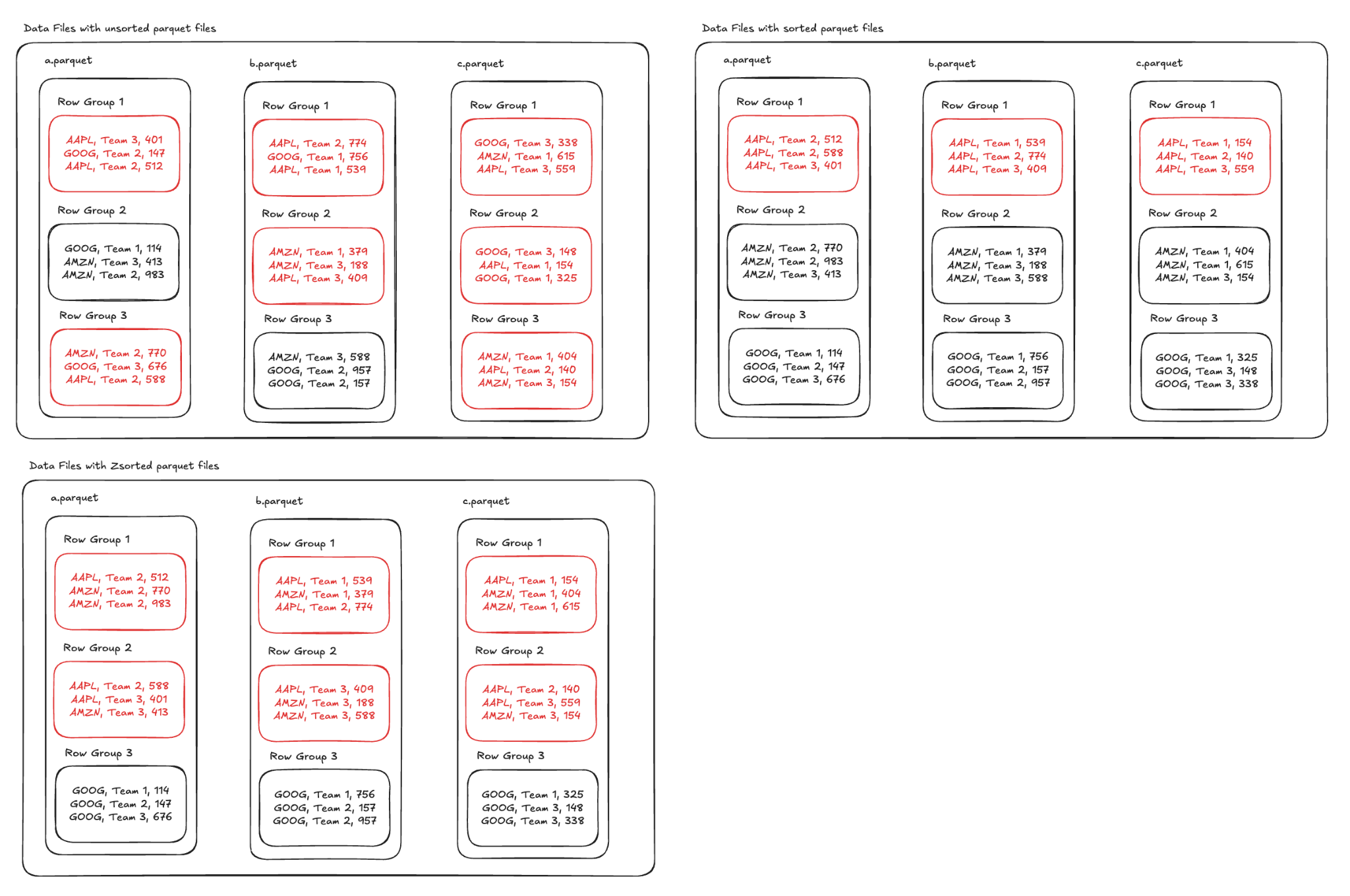
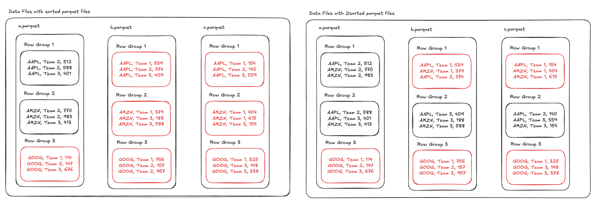
If the data is not optimally ordered, then the rows where symbol = ‘AAPL’ may be in numerous row groups. This means the query engines must check all those row groups. One simple optimization involves sorting the Parquet file by (symbol, team). This significantly reduces the number of row groups the query engines need to inspect.
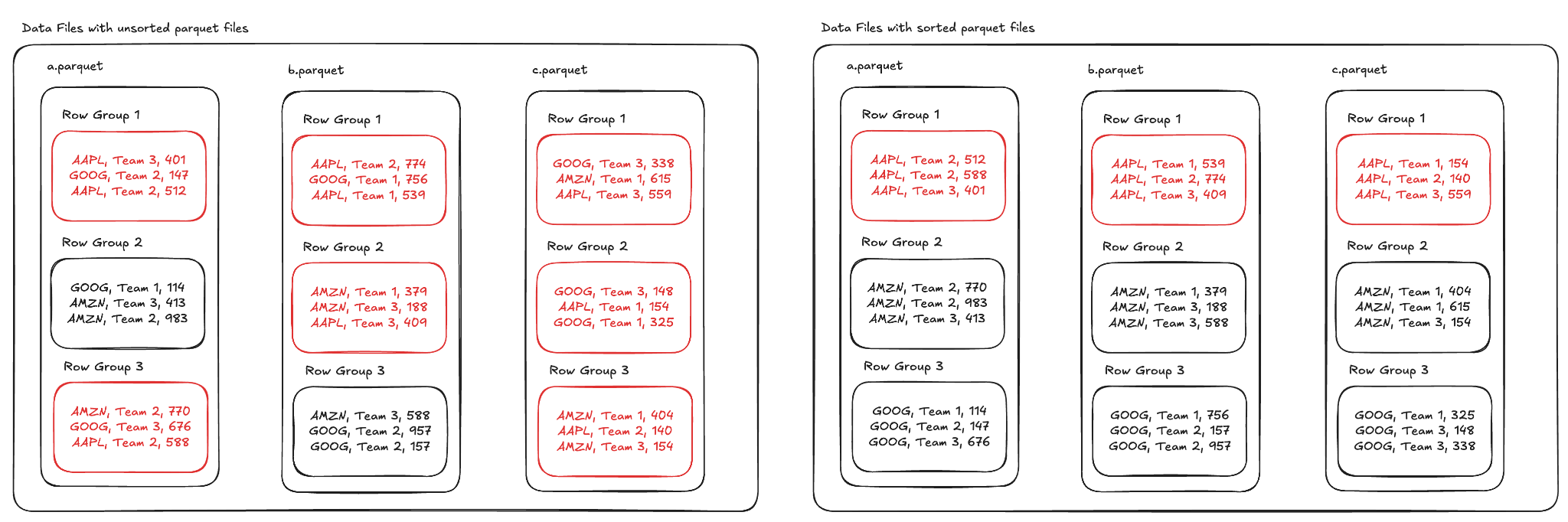
Problem
Although the optimization above performs strongly on symbol filters, it falls extremely short on team filters. Despite the multi-column sort, the layout above would be ill-suited for a WHERE team = ‘Team 1’ query, as lower-priority sort columns are still scattered throughout the parquet files:
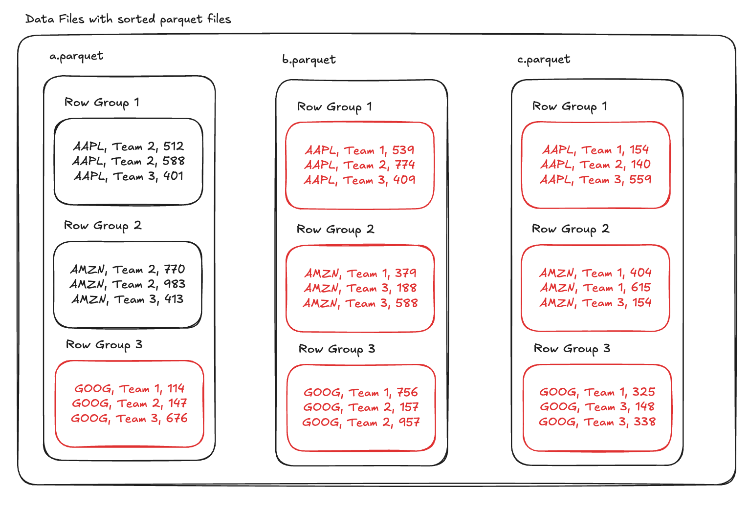
Thus, I needed to build an algorithm that could balance query performance across many columns.
Z-Ordering
We had the idea to use Z-ordering, which would have more evenly distributed “sortedness” across multiple columns. Z-ordering is a known algorithm that some table engines provide out-of-box, such as Dremio. However, since HRT has a bespoke data ingestion pipeline for Iceberg tables, I had to write my own implementation that rewrites a parquet file to be Z-ordered.
Z-order
To calculate the Z-order of a row, you take the values, convert them into a lexicographically sortable format, and then interleave the bits of each value. The result is a single sortable value that approximately preserves locality across all of the columns, so rows with similar combinations of values tend to end up near one another. In fact, the name becomes much clearer when one visualizes a Z-ordering across two continuous integer columns:
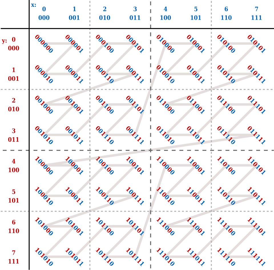
Going back to the more concrete example, implementing a Z-ordering algorithm provides read performance improvements for both symbol and team filtering:
Impact
Although we walked through a toy example, Z-ordering really shines as one scales up the size of the datasets. At HRT, we regularly build petabyte-scale Iceberg datasets, where read performance can greatly increase productivity and the user experience for our researchers. A single query on a small subset of (date, asset_class, team, symbol) columns of some of our tables might require opening hundreds of gigabytes of parquet. Using Z-ordering on the most commonly filtered columns, we saw a 20-25% improvement in average query time.
Stall Monitor
By Hadrian Reppas
Background
A typical automated trading system is driven by market events, such as an order placed on an exchange or a trade occurring. These event-driven systems encounter production issues due to “stalls,” where the program takes too much time to process an event and can’t perform its other duties. To detect these stalls, we determine how long it takes to handle each event:
auto start = Time::now();

handleEvent();

auto duration = Time::now() - start;
if (duration > WarnThreshold) {
    log.warn("handling event took %s", duration);
}Stalls typically happen when an unexpected expensive operation takes place on the critical path to process an event. There are many possible such operations: DNS resolutions, large heap allocations, or even reading config files from NFS. But the current approach offers little visibility into what actually caused a particular stall. We’d like to:
- Gather detailed information when a stall occurs.
- Avoid introducing any measurable overhead during normal execution. We can tolerate some overhead once a stall has been detected since the process is already taking far longer than it should.
Architecture
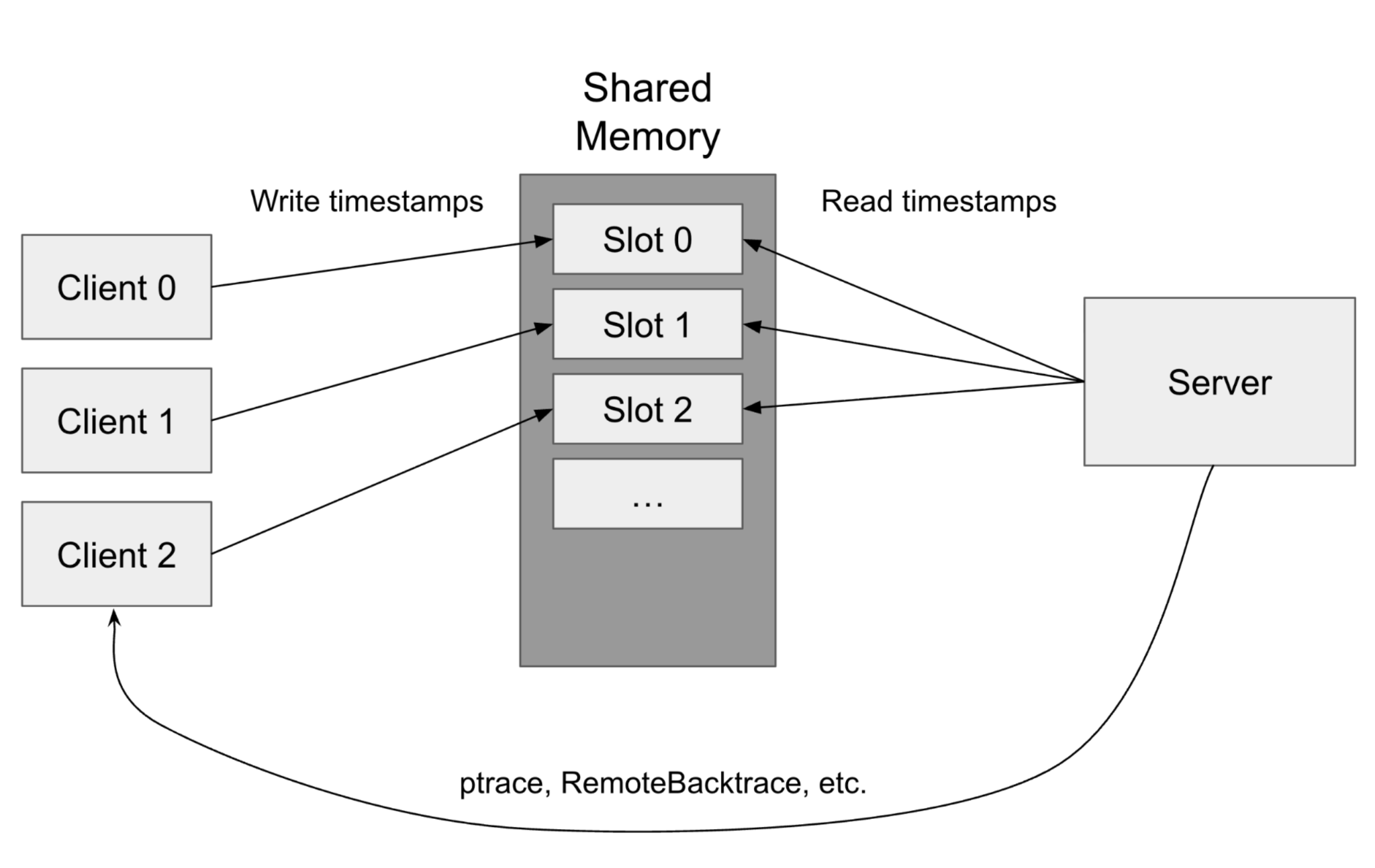
Our solution is a stall monitor server that runs on each host. Latency-sensitive processes on that host can register with the stall monitor to be given a slot in shared memory. They write the current time to their slot before handling each event and clear it after they finish. The server repeatedly checks the slots for stale timestamps, which indicate a stall. This offloads the work of detecting stalls to the server, which runs in its own process. Once a stall is detected, the server can attach to the stalled process to collect information about the stall.
The Client
We provide a lightweight Client class that each client process instantiates to register with the stall monitor. Apart from a one-time handshake with the server during initialization, the Client class does only two things:
- Writes the current time to its shared memory slot (using rdtsc and a non-temporal store).
- Clears the slot after handling the event (also with a non-temporal store).
The non-temporal stores bypass the cache to avoid polluting it. In benchmarks, the slowdown from these two operations was negligible relative to typical event processing latency.
The Server
When the server detects a stall, it can:
- Log the stall. This is the simplest option with the lowest overhead, but it provides no more information than the original timing-based approach.
- Log the instruction pointer. This can point us towards a slow function or syscall but requires briefly pausing the client process, which introduces some overhead.
- Collect a full backtrace using libunwind. This also requires briefly pausing the client. To minimize performance impact, we copy the client’s stack into the server and perform a remote unwind in the server’s own address space.
- Record a full instruction trace using Intel Processor Trace. Intel PT lets us reconstruct the exact sequence of instructions executed during the stall. It offers the most information with relatively modest overhead.
Testing
To verify the reliability of the stall monitor, we can set up parallel test clients that stall for randomized intervals and durations, and observe the server’s output.
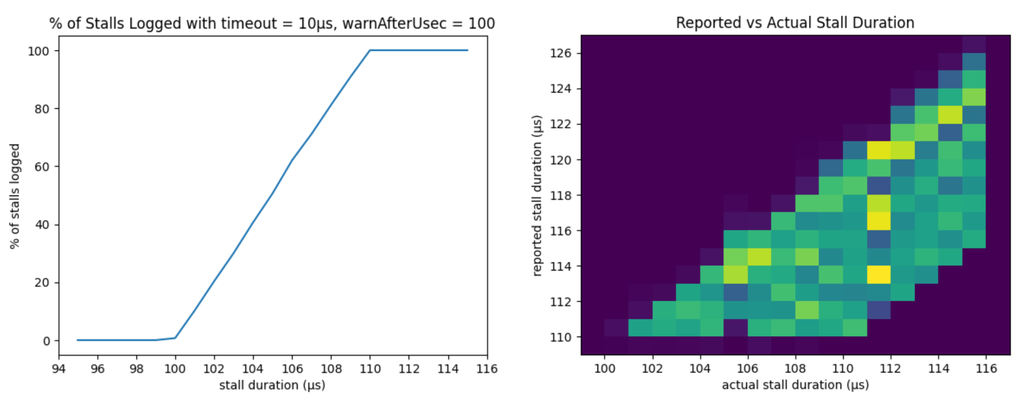
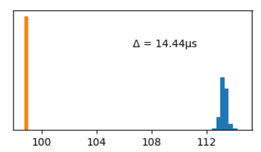
To profile the overhead of the server stopping the client process to collect information about the stall, we can measure the duration of the stall in the client with and without the stall monitor. For 100 microsecond stalls on a production trading machine, we observe the stall is ~15 microseconds longer when the server copies the client’s stack to unwind into a stack trace.
By offloading stall detection to a separate process and using efficient communication via shared memory, we can now collect detailed traces of latency spikes with minimal impact on latency during production trading.